Plain Network(단순히 Layer을 깊게 쌓음)에서 발생하는 Vanishing Gradient(기울기 소실), Overfitting(과적합) 등의 문제를 해결하기 위해 ReLU, Batch Nomalization 등 많은 기법이 있습니다.
ILSVRC Challenge2021년 3월 24일 기준 인용
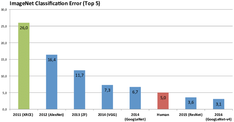
ILSVRC 대회에서 2015년, 처음으로 Human Recognition보다 높은 성능을 보인 것이 ResNet입니다.
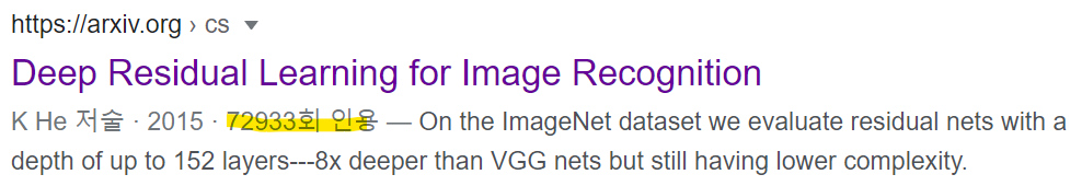
그 위용은 무지막지한 논문 인용 수로 확인할 수 있습니다.
그렇기 때문에 ResNet은 딥러닝 이미지 분야에서 바이블로 통하고 있습니다.
Plain Netwrok Vs ResNet
Plain Network는 단순히 Convolution 연산을 단순히 쌓는다면, ResNet은 Block단위로 Parameter을 전달하기 전에 이전의 값을 더하는 방식입니다.
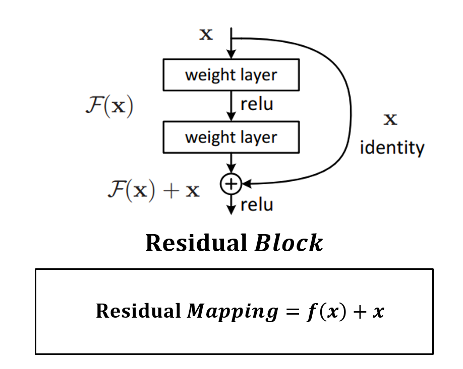
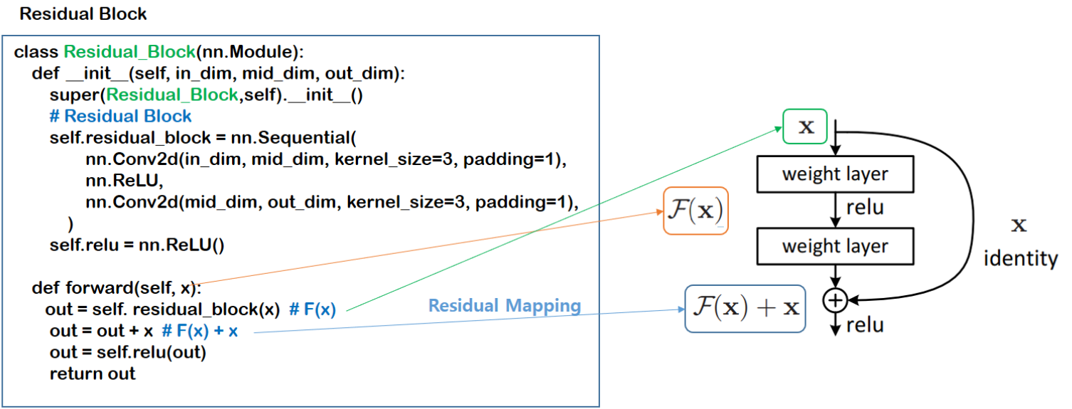
Residual Block
F(x) : weight layer => relu => weight layer
x : identity
weight layer들을 통과한 F(x)와 weight layer들을 통과하지 않은 x의 합을 논문에서는 Residual Mapping 이라 하고, 그림의 구조를 Residual Block이라 하고, Residual Block이 쌓이면 Residual Network(ResNet)이라고 합니다.
Residual Mapping은 간단하지만, Overfitting, Vanishing Gradient 문제가 해결되어 성능이 향상됐습니다.
그리고 다양한 네트워크 구조에서 사용되며, 2017년 ILSVRC을 우승한 SeNet에서 사용됩니다. ( 이 글을 쓴 이유이기도 합니다. )
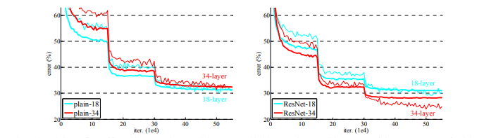
Plain Network VS ResNet (Error)
Residual Block
class Residual_Block(nn.Module):
    def __init__(self, in_dim, mid_dim, out_dim):
        super(Residual_Block,self).__init__()
        # Residual Block
        self.residual_block = nn.Sequential(
                nn.Conv2d(in_dim, mid_dim, kernel_size=3, padding=1),
                nn.ReLU,
                nn.Conv2d(mid_dim, out_dim, kernel_size=3, padding=1),
            )
        self.relu = nn.ReLU()

    def forward(self, x):
       out = self. residual_block(x)  # F(x)
        out = out + x  # F(x) + x
        out = self.relu(out)
        return out
그리고 Residual Block 소개 후 BottleNeck이 나옵니다. 아래 글을 참고하시면 좋을 것 같습니다.
CNN에서 CIR Featur을 추출, Redundant information을 제거하고, LSTM을 이용하여 분류합니다.
( CNN+stacked-LSTM Accuracy : 82.14% )
Model StructureCNN StructureLSTM StructureResult
Implemnet ( Dataset : df_uwb_data 준비 )
1. Import
import torch
import torch.nn as nn
import torch.optim as optim
from torch.utils.data import DataLoader, TensorDataset
from torch.utils.tensorboard import SummaryWriter

from sklearn.model_selection import train_test_split
from sklearn.metrics import accuracy_score, precision_score, recall_score, f1_score

import numpy as np
import pandas as pd
import matplotlib.pyplot as plt

import time
import random

import uwb_dataset

print("Pytorch Version :", torch.__version__)  # Pytorch Version : 1.7.1+cu110
writer = SummaryWriter('runs/UWB_CIR_Classfication')

%matplotlib inline
import numpy as np
import pandas as pd
import pandas_datareader.data as pdr
import matplotlib.pyplot as plt

import datetime

import torch
import torch.nn as nn
from torch.autograd import Variable

import torch.optim as optim
from torch.utils.data import Dataset, DataLoader
no module pandas_datareaderno module named 'pandas_datareader'
pandas가 깔려 있는데, 위 문구가 뜬다면 pip install pandas_datareader로 다운로드합니다.
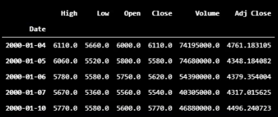
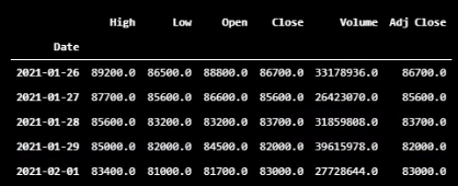
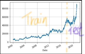
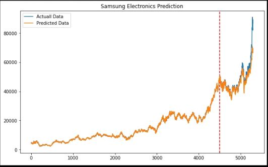
그리고 학습된 모델이 성능을 확인하기 위해서 위 데이터(현재 약 5296개)를 Train(학습하고자 하는 데이터)를 0부터 4499까지, Test(성능 테스트하는 데이터)는 4500부터 5295개 까지 데이터로 분류합니다.
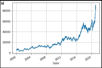
오늘자 대략, 노란색 선 정도까지 데이터를 가지고 학습을 하고, 노란색 선 이후부터 예측을 할 것입니다.
과연 내려가고 올라가는 포인트를 잘 예측할 수 있을지 궁금합니다.
3. 데이터셋 준비하기
"""
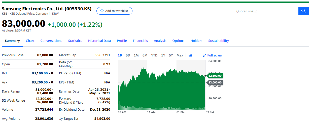
저도 주식을 잘 모르기 때문에 참고해주시면 좋을 것 같습니다.
open 시가
high 고가
low 저가
close 종가
volume 거래량
Adj Close 주식의 분할, 배당, 배분 등을 고려해 조정한 종가
확실한건 거래량(Volume)은 데이터에서 제하는 것이 중요하고,
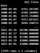
Y 데이터를 Adj Close로 정합니다. (종가로 해도 된다고 생각합니다.)
"""
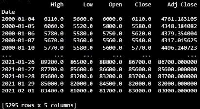
X = df.drop(columns='Volume')
y = df.iloc[:, 5:6]
print(X)
print(y)
Xy
"""
학습이 잘되기 위해 데이터 정규화
StandardScaler 각 특징의 평균을 0, 분산을 1이 되도록 변경
MinMaxScaler 최대/최소값이 각각 1, 0이 되도록 변경
"""
from sklearn.preprocessing import StandardScaler, MinMaxScaler
mm = MinMaxScaler()
ss = StandardScaler()
X_ss = ss.fit_transform(X)
y_mm = mm.fit_transform(y)
# Train Data
X_train = X_ss[:4500, :]
X_test = X_ss[4500:, :]
# Test Data
"""
( 굳이 없어도 된다. 하지만 얼마나 예측데이터와 실제 데이터의 정확도를 확인하기 위해
from sklearn.metrics import accuracy_score 를 통해 정확한 값으로 확인할 수 있다. )
"""
y_train = y_mm[:4500, :]
y_test = y_mm[4500:, :]
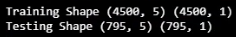
print("Training Shape", X_train.shape, y_train.shape)
print("Testing Shape", X_test.shape, y_test.shape)
numpy 형태 : 이 상태에서는 학습이 불가능.
"""
torch Variable에는 3개의 형태가 있다.
data, grad, grad_fn 한 번 구글에 찾아서 공부해보길 바랍니다.
"""
X_train_tensors = Variable(torch.Tensor(X_train))
X_test_tensors = Variable(torch.Tensor(X_test))

y_train_tensors = Variable(torch.Tensor(y_train))
y_test_tensors = Variable(torch.Tensor(y_test))

X_train_tensors_final = torch.reshape(X_train_tensors,   (X_train_tensors.shape[0], 1, X_train_tensors.shape[1]))
X_test_tensors_final = torch.reshape(X_test_tensors,  (X_test_tensors.shape[0], 1, X_test_tensors.shape[1]))

print("Training Shape", X_train_tensors_final.shape, y_train_tensors.shape)
print("Testing Shape", X_test_tensors_final.shape, y_test_tensors.shape)
학습할 수 있는 형태로 변환하기 위해 Torch로 변환
4. GPU 준비하기 (없으면 CPU로 돌리면 됩니다.)
device = torch.device("cuda:0" if torch.cuda.is_available() else "cpu")  # device
print(torch.cuda.get_device_name(0))
5. LSTM 네트워크 구성하기
class LSTM1(nn.Module):
  def __init__(self, num_classes, input_size, hidden_size, num_layers, seq_length):
    super(LSTM1, self).__init__()
    self.num_classes = num_classes #number of classes
    self.num_layers = num_layers #number of layers
    self.input_size = input_size #input size
    self.hidden_size = hidden_size #hidden state
    self.seq_length = seq_length #sequence length

    self.lstm = nn.LSTM(input_size=input_size, hidden_size=hidden_size,
                      num_layers=num_layers, batch_first=True) #lstm
    self.fc_1 =  nn.Linear(hidden_size, 128) #fully connected 1
    self.fc = nn.Linear(128, num_classes) #fully connected last layer

    self.relu = nn.ReLU()

  def forward(self,x):
    h_0 = Variable(torch.zeros(self.num_layers, x.size(0), self.hidden_size)).to(device) #hidden state
    c_0 = Variable(torch.zeros(self.num_layers, x.size(0), self.hidden_size)).to(device) #internal state
    # Propagate input through LSTM

    output, (hn, cn) = self.lstm(x, (h_0, c_0)) #lstm with input, hidden, and internal state

    hn = hn.view(-1, self.hidden_size) #reshaping the data for Dense layer next
    out = self.relu(hn)
    out = self.fc_1(out) #first Dense
    out = self.relu(out) #relu
    out = self.fc(out) #Final Output

    return out
위 코드는 복잡해 보이지만, 실상 하나씩 확인해보면 굉장히 연산이 적은 네트워크입니다.
시계열 데이터이지만, 간단한 구성을 위해 Sequence Length도 1이고, LSTM Layer도 1이기 때문에 굉장히 빨리 끝납니다. 아마 본문 작성자가 CPU환경에서도 쉽게 따라 할 수 있게 간단하게 작성한 것 같습니다.
num_epochs = 30000 #1000 epochs
learning_rate = 0.00001 #0.001 lr

input_size = 5 #number of features
hidden_size = 2 #number of features in hidden state
num_layers = 1 #number of stacked lstm layers

num_classes = 1 #number of output classes
for epoch in range(num_epochs):
  outputs = lstm1.forward(X_train_tensors_final.to(device)) #forward pass
  optimizer.zero_grad() #caluclate the gradient, manually setting to 0

  # obtain the loss function
  loss = loss_function(outputs, y_train_tensors.to(device))

  loss.backward() #calculates the loss of the loss function

  optimizer.step() #improve from loss, i.e backprop
  if epoch % 100 == 0:
    print("Epoch: %d, loss: %1.5f" % (epoch, loss.item()))