반응형

안녕하세요.


주피터 노트북 개인 딥러닝 서버 만들기 2편입니다.

이번 글은 주피터 노트북을 좀 더 유용하고 보기 좋게 만들기 위한 편입니다. 굳이 안 하시고 넘어가셔도 무방합니다.


~ 1. 주피터 노트북 테마 ~

저는 주피터 노트북 기본 테마를 별로 좋아하지 않습니다. 현재 제가 다니고 있는 연구실은 정부에서 지원하는 딥러닝 서버를 주피터 노트북으로 이용하고 있습니다. 저만 사용하는 것이 아니기 때문에, 기본 테마로 뒀습니다. 


하지만 이 딥러닝 서버는 오로지 저만을 위한 서버이기 때문에 테마를 바꾸겠습니다. 


anaconda prompt를 들어가 pip install jupyterthemes 를 입력해 테마 패키지를 설치합니다.

pip install jupyterthemes # 주피터 노트북 테마 패키지 설치
jt -l # 테마 목록 출력

"""
Available Themes:
   chesterish
   grade3
   gruvboxd
   gruvboxl
   monokai
   oceans16
   onedork
   solarizedd
   solarizedl
"""

저는 테마 grade3이 제일 좋아합니다. 

jt -t grade3 -T -N
-T : 툴바 보이게 설정
-N : 제목 보이게 설정


툴바는 무조건 있는게 편합니다. 제목은 내가 현재 어떤 파일을 편집하는지 알기 편하고, 제목을 누르면 수정할 수 있어 편합니다. 이 정도 설정하시면 문제없습니다. 폰트 사이즈나 다양한 설정이 있지만 그건 구글에 치면 많은 블로그가 있습니다.

툴바
제목
jt -t grade3 -T -N


~ 2. 주피터 노트북 확장 프로그램 ~

확장프로그램은 사람들이 추천하는 것을 사용하면 편합니다. 아래 블로그 분께서 추천하시는 것들을 하시면 편합니다. 

https://www.rlee.ai/jupyter/jupyter-notebook-exntesions


주피터 노트북 확장 프로그램 사용하기

jupyter_contrib_nbextensions는 몇십 가지의 확장 프로그램을 모아둔 패키지입니다. 그 중에서 특히 많이 찾으실 만한 확장 프로그램들은 다음과 같습니다.

www.rlee.ai

개인적으로 몇 개를 더 추천드립니다.

2.1. Code prettify

제목 그대로 코드를 이쁘게 정리하는 툴입니다. 동작에는 영향을 끼치진 않습니다. 

2.2. Variable Inspector

매트랩의 작업 공간처럼, 변수들을 전체적으로 확인할 수 있습니다.

2.3. Execute Time

실행된 셀의 걸린 시간을 알려줍니다. 

executed in 15ms, finished 23:14:02 2021-07-16


그 외에 많은 툴이 있으니 찾아보시길 바랍니다. 설명도 자세히 나와 있기 때문에 커스터마이징 하기 좋습니다.

Nbextensions 클릭
설정


~ 3. DDNS ~

아래 블로그 분께서 DDNS에 대해 잘 설명해주셨습니다. ( ipTIME 공유기는 무료로 가능합니다. )

IP를 외우고 다니는 사람은 없습니다. DNS라 하여 IP의 또 다른 이름이라고 생각하시면 좋습니다. 

ex) www. naver. com

우리도 IP 대신 DNS를 사용하는 것입니다. 

https://luckygg.tistory.com/271


[ipTIME] DDNS 설정으로 외부에서 쉽게 공유기에 접속하기

DDNS(Dynamic DNS)란? 우선 DDNS를 이해하기 전에 DNS(Domain Name system)를 이해해야 합니다. 우리는 웹 브라우저에서 네이버나 구글에 접속하기 위해 www.naver.com 또는 www.google.com이라는 주소로 접속합니..

luckygg.tistory.com


ipTIME일 경우...

{사용자 지정}.iptime.org:{포트번호}


그런데 하나 이상한 부분이 있지 않나요?


보통 Naver나 Google을 브라우저에 입력할 때, 포트 번호를 적으시나요?

Naver를 접속할 때, 우리는 브라우저에 www.naver.com 입력합니다. 포트 번호는 어디 갔을까요?

이유는 간단합니다. http 포트번호는 80번으로, Well Known Port 번호입니다. 말 그대로 잘 알려진 포트번호입니다. 브라우저 내에서 생략되어 알아서 80번으로 접근합니다. 그렇기 때문에 www.naver.com:80 으로 들어가도 잘 동작합니다.


참고로 알아도 좋고, 몰라도 좋습니다.


~ 4. WoL ~

WoL은 Wake on LAN의 약자입니다. 말 그대로 원격으로 LAN을 통해 내 컴퓨터에 신호를 주어 깨운다는 뜻입니다. 항상 PC를 켜놓을 수 없기 때문에, 필요할 때 모바일로 내 컴퓨터를 켤 수 있습니다. 

WoL 같은 경우는 메인보드, 랜 카드 지원 호환성을 알아야 합니다. ( 보통 요즘 PC들은 거의 지원합니다. ) 


아래 블로그 분께서 깔끔히 정리해놓은 것이 있으니, 아래 것을 참고하시길 바랍니다.

https://luckygg.tistory.com/277


[ipTIME] WOL 어플로 어디서든 내 컴퓨터 전원 켜기

WOL이란? WOL은 Wake On Lan의 약자로, 특정 네트워크에 연결되어 있는 컴퓨터의 전원을 LAN을 통해 원격으로 켜는 기능입니다. WOL 설정만 되어 있다면 스마트폰으로 언제 어디서든 쉽게 집 또는 회사

luckygg.tistory.com


저처럼 ASUS 메인보드라면, 아래 블로그 참고하시길 바랍니다. 

https://intunknown.tistory.com/576


asus 메인보드 wol 설정 [bios]

asus 메인보드 wol 설정 [bios] 안녕하세요. 오늘은 wol을 하기 위해 바이오스를 설정해보려고 합니다. wol에 대한 간단한 설명. asus 메인보드 바이오스 설정. wol에 대한 간단한 설명. 이거 검색해서 올

intunknown.tistory.com


다음 글은 Pytorch GPU 버전을 설치하고, 딥러닝 SeNet 가볍게 하나 돌려 보겠습니다. 

https://coding-yoon.tistory.com/154


주피터 노트북 개인 딥러닝 서버 만들기 ! (3) with Window10, Pytorch

안녕하세요. 만약 여기까지 따라 오셨다면 90% 정도 성공입니다. 나머지 10%는 Pytorch만 설치하면 됩니다. 굉장히 간단합니다. 아래 Pytorch 공식 사이트를 들어 갑니다. https://pytorch.org/ PyTorch An open s.

coding-yoon.tistory.com


728x90
반응형
반응형


이번에 컴퓨터를 맞추면서 그래픽카드 RTX 2060 super를 구매했습니다. 저만의 딥러닝 서버를 만들어 놓으면 어디서든 야외에서 노트북으로 가볍게 작업할 수 있습니다. ( 얼마나 작업을 할지 모르지만, 없는 것보단 나을 것 같습니다. )


천천히 따라오시면 누구나 간단히 주피터 노트북을 이용해 서버를 열 수 있습니다. 


~ 1. ANACONDA 설치 ~

우선, 주피터 노트북을 설치합니다. 


https://www.anaconda.com/products/individual


Anaconda | Individual Edition

Anaconda's open-source Individual Edition is the easiest way to perform Python/R data science and machine learning on a single machine.

www.anaconda.com


Anaconda를 설치합니다. 2021.07.14 기준 Python3.8주피터 노트북이 설치됩니다. 

( 따로 경로는 설정할 필요는 없기 때문에, 기본 경로 설정으로 설치합니다. )


설치를 완료하면.


위 그림처럼 설치된 파일들을 확인할 수 있습니다. 


우리에게 필요한 것은 Anaconda Prompt (anaconda3)Jupyter Notebook (anaconda3)입니다.


~ 2. 주피터 노트북 설정을 위한 파일 생성 ~

Anaconda Prompt를 들어가서 아래의 명령어를 입력합니다.

jupyter notebook --generate-config

위 명령어는 주피터 노트북의 설정 파일(. py)을 생성하는 의미입니다. 

Window User -> C:/Users/"사용자 이름"/.jupyter
Linux User -> /home/"사용자 이름"/.jupyter


저는 주피터 노트북 테마, 확장 프로그램을 건드렸기 때문에 많은 파일들이 있지만, 처음 설정하시는 분들께서는jupyter_notebook_config.py만 있습니다.


저처럼 코드 편집기가 없으시면 메모장으로 들어가서 작업하시면 됩니다.


코드를 편집하기 전에, 자신의 로컬(private) IP와 포트포워딩을 위한 포트 번호를 지정해야 합니다.


~ 3. IP 확인, 고정, 포트포워딩 ~

3.1. IP 확인, 고정 (공인 IP, 사설 IP)

우선, 간단히 IP의 종류에는 두 가지가 있습니다.

외부에서 받아 오는 공인(Public) IP (외부),  공유기에서 나눠주는 로컬(private) IP (내부)가 있습니다.


1. 공인 IP

공인 IP를 확인하는 방법은 여러 가지가 있습니다. 간단히 네이버에서 내 아이피 보기를 검색하시면 자신의 공인 IP를 확인할 수 있습니다.

첫번 째 방법.


두 번째, 192.168.0.1( 공유기 관리자 모드 )를 url을 통해 들어간다. 로그인 창이 뜨는데, 처음 자신이 설정한 아이디와 비밀번호를 입력한다. ( 잊었을 시, 리셋 )


저는 ipTIME을 사용합니다. ( 공유기마다 환경이 다릅니다. ) ipTIME은 외부 IP 주소라고 바로 확인할 수 있습니다.


공인 IP를 알아야 하는 이유는 나중에 외부에서 주피터 노트북 서버를 접근하기 위해 필요합니다. 

( 간단히, 위 공인 IP를 우리가 구매했기 때문에, 우리가 네이버에서 확인한 공인 IP는 유일무이합니다. 하지만, 사설 IP는 공유기가 랜덤 하게( 혹은 우리가 직접 ) 만들어 주기 때문에, 굉장히 많습니다. ) 


2. 사설 IP

쉽게 설명하자면, 192.168.0.xx의 규칙을 가지는 IP는 모두 사설 IP입니다. cmd에서 ipconfig를 입력하면 됩니다.

혹은, 공유기 관리자 모드를 들어가 확인하는 것입니다. 


① 보통 사설 IP는 자동으로 할당되어 IP가 박스 1의 IP주소 대여 범위 안에서 수시로 변경됩니다. 오늘은 cmd에서 확인한 것처럼 192.168.0.15이지만, 내일은 192.168.0.16으로 IP가 변경될 수 있습니다. 


박스 2의 사용 중인 IP 주소 정보를 보시면, 현재 와이파이 등 공유기에 물려 있는 기기들을 확인할 수 있습니다. 저는 192.168.0.15를 그대로 사용하겠습니다.


③  현재 사용 중인 IP를 클릭하면 자동으로 IP, mac 주소까지 입력되니 설명은 자신이 구별할 수 있게 적고 수동 등록합니다. 그러면 박스 3에서처럼 리스트에 저장되어 고정됩니다.

약간의 이해를 위해 태블릿으로 저희 집 네트워크 상태를 그려 봤습니다. 

우리들이 접근하고자 하는 서버는 50.0.x.x192.168.0.15 서버입니다. 하지만, 우리가 브라우저에 IP를 치고 들어갈 때, 저런 식으로 입력하나요? 아닙니다.


그래서 나온 것이 포트 번호입니다. ( 정확히는 이 때문에 나온 것은 아닙니다. IP는 네트워크(3) 계층, Port 번호는 전송(4) 계층으로 네트워크 구조를 자세히 알아야 합니다. 통신 전공자가 아니라면, 이 정도만 이해해도 충분하다고 생각이 듭니다. ) 우리가 사용하고자 하는 50.0.x.x192.168.0.15 대신 50.0.x.x:{port number}를 입력합니다. (대표적으로 포트번호 http는 80, ssh는 22, 주피터 노트북 서버의 디폴트 포트번호는 8888입니다.  주피터 노트북을 아무 설정 없이 실행하면, localhost:8888로 들어가게 됩니다. )


8888로 그대로 사용해도 됩니다.  우리들은 보안 전공이 아니지만, 적어도 포트번호를 다르게 써서 그나마 안전하게 접근할 수 있도록 할 예정입니다. 

3.2. 포트포워딩


포트포워딩은 공유기에게 문을 열어주는 역할을 합니다. 우리가 주피터 노트북 기본 포트번호가 8888인 것은 알지만, 공유기는 알지 못합니다. 이를 공유기에게 지정하는 것입니다. 만약 50.0.x.x에서 포트번호 8888을 만났다면, 여기로 가세요. 정도로 이해하시면 될 것 같습니다. 


우리는 기본 주피터 노트북 포트 번호를 그대로 사용하지 않고 jupyter_notebook_config.py에서 포트 번호를 바꿔줍니다. 포트번호는 0부터 65535까지 범위(16bit = 2^16)를 사용합니다. 위에서 언급했듯이, HTTP는 80, SSH는 22 등 이미 사용되고 포트 번호가 있습니다. Well Known Port Number이라고 합니다. 이 숫자들을 피해 저는 3333이라는 포트 번호를 주피터 노트북 포트 번호로 사용하겠습니다. 다른 숫자를 쓰고 싶으신 분은 위 유의사항을 피해 사용하시면 됩니다. 

저와 같은 ipTIME 공유기라면, 저를 따라 하시면 됩니다. 하나씩 설명해드리겠습니다.

규칙 이름 : 사용자 마음대로

IP 주소 : 자신이 딥러닝 서버로 만들고자 하는 로컬 IP

프로토콜 : TCP

외부포트 : 7777 ( 그림에서 설명하겠습니다. )

내부포트 : 3333 ( 주피터 노트북 서버 포트 번호) 


어렵게 생각하실 필요 없습니다. 


50.0.x.x:7777로 접근했다면...

"7777포트는 3333포트를 가리키는구나."

50.0.x.x:3333으로 길을 안내해줍니다. 3333포트는 192.168.0.15의 주피터 노트북 서버를 가리킵니다.


만약 나는 8888 그대로 사용하겠다 싶으시면, 외부포트 8888, 내부포트 8888 그대로 사용하시면 됩니다. 솔직히 문제되진 않습니다. 누가 개인 서버를 털겠습니까? 털어갈 것도 없으니...


~ 4. 주피터 노트북 설정 ~


Anaconda Prompt에서 jupyter_notebook_config.py를 위에서 생성했습니다.  경로는 아래와 같이 

Window User -> C:/Users/"사용자 이름"/.jupyter
Linux User -> /home/"사용자 이름"/.jupyter

jupyter_notebook_config.py를 메모장 혹은 코드 편집기로 열어 줍니다. 아마 알 수 없는 코드들이 작성되있습니다. 하지만 대부분이 주석이기 때문에 실제 코드는 얼마되지 않으니 걱정안하셔도 됩니다. ( 파이썬 주석은 #입니다. 주석은 설명입니다. )


4.1. 주피터 노트북 포트번호 설정

## The port the notebook server will listen on (env: JUPYTER_PORT).
#  Default: 8888
c.NotebookApp.port = 3333 # 자신이 원하는 포트 번호

4.2. 주피터 노트북 비밀번호 설정

## Hashed password to use for web authentication.
#  
#  To generate, type in a python/IPython shell:
#  
# from notebook.auth import passwd 
# passwd()
#
#  The string should be of the form type:salt:hashed-password.
#  Default: ''
# c.NotebookApp.password = password

아마 기본적으로 위 같이 주석처리가 되있을 것입니다. 아래와 같이 주석을 해제하고 자신이 원하는 비밀번호를 작성하시면 됩니다. jupyter_notebook_config.py이 파이썬 코드이기 때문에 괜찮습니다.


## Hashed password to use for web authentication.
#  
#  To generate, type in a python/IPython shell:
#  
from notebook.auth import passwd 
password = passwd('자신이 원하는 비밀번호')  # 기본으로 argon2를 사용
# password = passwd('자신이 원하는 비밀번호', 'sha256')  # option : 'sha1', 'sha256'...
#  
#  The string should be of the form type:salt:hashed-password.
#  Default: ''
c.NotebookApp.password = password

4.3. 주피터 노트북 IP 설정

## The IP address the notebook server will listen on.
#  Default: 'localhost'
c.NotebookApp.ip = '192.168.0.15'

4.4. 주피터 노트북 외부 접속 허용 설정

#  Takes precedence over allow_origin_pat.
#  Default: ''
c.NotebookApp.allow_origin = '*'

4.5. 주피터 노트북 시작시 브라우저 자동 실행 안함

## Whether to open in a browser after starting. The specific browser used is
#  platform dependent and determined by the python standard library `webbrowser`
#  module, unless it is overridden using the --browser (NotebookApp.browser)
#  configuration option.
#  Default: True
c.NotebookApp.open_browser = False

4.6. 주피터 노트북 작업 경로 설정

의외로 작업 경로 설정하는 것이 복병이었습니다. 코드 상에서 작업 경로를 제대로 입력하더라도 Home 경로로 이동해버립니다. 아래 블로그 분께서 친절하게 문제점을 알려주시니 그대로 보고 따라 하시면 됩니다.

https://wonderbout.tistory.com/50


주피터 노트북(Jupyter Notebook) 시작 폴더 변경

주피터 노트북을 실행하면 최초 폴더 경로가 사용자 폴더로 돼있습니다. 다른 폴더에서 작업을 하려 해도 하위 폴더 외에는 이동할 수가 없습니다. 예를 들어 제 경우 D 드라이브에 있는 특정 폴

wonderbout.tistory.com

빨간 박스 다 지우기

## The directory to use for notebooks and kernels.
#  Default: ''
c.NotebookApp.notebook_dir = '자신이 원하는 경로'


~ 5. 마무리 ~

네트워크 설정과 주피터 노트북 설정을 모두 마쳤습니다. 한 번 테스트하겠습니다. 

브라우저에 외부 IP:포트번호처럼 입력해서 들어가시면 됩니다. 

ex) 50.0.x.x:7777

PC에서 성공

다른 기기에서 접속해보겠습니다.


성공


주피터 노트북으로 외부 접속을 성공했습니다. 다음 글은 주피터 테마, 확장 프로그램, DDNS, WoL입니다.

https://coding-yoon.tistory.com/153


주피터 노트북 개인 딥러닝 서버 만들기 ! (2)

안녕하세요. 주피터 노트북 개인 딥러닝 서버 만들기 2편입니다. 이번 글은 주피터 노트북을 좀 더 유용하고 보기 좋게 만들기 위한 편입니다. 굳이 안 하시고 넘어가셔도 무방합니다. ~ 1. 주피

coding-yoon.tistory.com


728x90
반응형
반응형

안녕하세요. 


Deep Learning은 대표적으로 분류 문제가 있으며, CNN의 튜토리얼은 MNIST, CIFAR10 분류로 가장 많이 소개됩니다. 

이진 분류는 Sigmoid를, 그 이상의 다중 분류는 Softmax를 사용하며, Softmax를 사용하기 위해 One-hot encoding을 해야 합니다. 

Sotfmax의 가장 중요한 점은 각 Class 간의 Probabilities(확률)의 합이 '1'입니다. 정답 Class가 1에 가까워지면, 자연스럽게 오답인 Class의 Probabilities는 0에 가까워지게 됩니다. 

One-hot encoding
Softmax

하지만 Pytorch는 One-hot encoding을 하지 않습니다. Pytorch 개발자들이 최대한 사람 친화적으로 개발을 할 수 있게끔 배려를 한 것 같습니다. 

One-hot encoding

그렇다면, Target n is out of bounds. 에러문은 왜 뜨는 것일까요?


이유는 간단합니다. 인덱스 오류랑 원리가 같습니다.


대게 class가 0부터 시작하지 않고, 1부터 시작해서 

Class가 20개라면, 0~19...

Class가 15개라면, 0~14...


만약, Class 5개에서, 1~5라면, 해결방법도 간단합니다. 


Data Type이 Numpy나 Tensor라면, y_data = y_data - 1을 해주면 쉽게 해결됩니다.

728x90
반응형
반응형

안녕하세요. 


Plain Network(단순히 Layer을 깊게 쌓음)에서 발생하는 Vanishing Gradient(기울기 소실), Overfitting(과적합) 등의 문제를 해결하기 위해 ReLU, Batch Nomalization 등 많은 기법이 있습니다. 
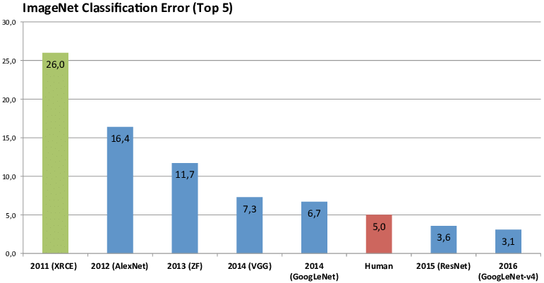
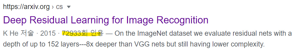
 

ILSVRC Challenge
2021년 3월 24일 기준 인용

ILSVRC 대회에서 2015년, 처음으로 Human Recognition보다 높은 성능을 보인 것이 ResNet입니다.

그 위용은 무지막지한 논문 인용 수로 확인할 수 있습니다. 


그렇기 때문에 ResNet은 딥러닝 이미지 분야에서 바이블로 통하고 있습니다. 


Plain Netwrok Vs ResNet

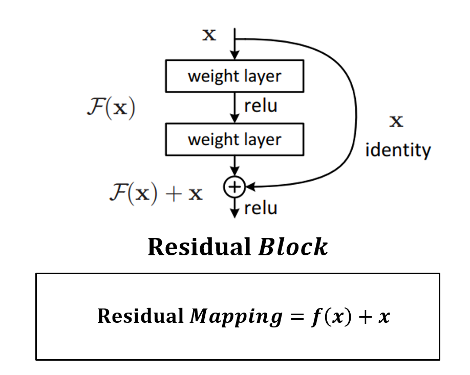
Plain Network는 단순히 Convolution 연산을 단순히 쌓는다면, ResNet은 Block단위로 Parameter을 전달하기 전에 이전의 값을 더하는 방식입니다. 
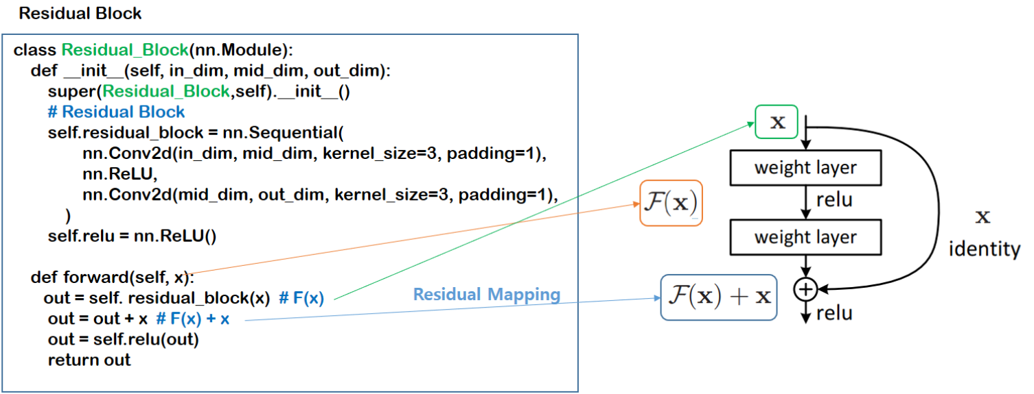
 

Residual Block

F(x) : weight layer => relu => weight layer 

x : identity


weight layer들을 통과한 F(x)와 weight layer들을 통과하지 않은 x의 합을 논문에서는 Residual Mapping 이라 하고, 그림의 구조를 Residual Block이라 하고, Residual Block이 쌓이면 Residual  Network(ResNet)이라고 합니다.

Residual Mapping은 간단하지만, Overfitting, Vanishing Gradient 문제가 해결되어 성능이 향상됐습니다.

그리고 다양한 네트워크 구조에서 사용되며, 2017년 ILSVRC을 우승한 SeNet에서 사용됩니다. ( 이 글을 쓴 이유이기도 합니다. ) 


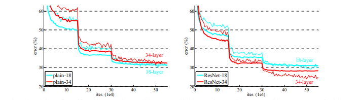
Plain Network VS ResNet (Error)


Residual Block

class Residual_Block(nn.Module):
    def __init__(self, in_dim, mid_dim, out_dim):
        super(Residual_Block,self).__init__()
        # Residual Block
        self.residual_block = nn.Sequential(
                nn.Conv2d(in_dim, mid_dim, kernel_size=3, padding=1),
                nn.ReLU,
                nn.Conv2d(mid_dim, out_dim, kernel_size=3, padding=1),
            )            
        self.relu = nn.ReLU()
                  
    def forward(self, x):
       out = self. residual_block(x)  # F(x)
        out = out + x  # F(x) + x
        out = self.relu(out)
        return out


그리고 Residual Block 소개 후 BottleNeck이 나옵니다. 아래 글을 참고하시면 좋을 것 같습니다. 

coding-yoon.tistory.com/116?category=825914


[딥러닝] DeepLearning CNN BottleNeck 원리(Pytorch 구현)

안녕하세요. 오늘은 Deep Learning 분야에서 CNN의 BottleNeck구조에 대해 알아보겠습니다. 대표적으로 ResNet에서 BottleNeck을 사용했습니다. ResNet에서 왼쪽은 BottleNeck 구조를 사용하지 않았고, 오른쪽은..

coding-yoon.tistory.com

ResNet 원문

arxiv.org/abs/1512.03385


Deep Residual Learning for Image Recognition

Deeper neural networks are more difficult to train. We present a residual learning framework to ease the training of networks that are substantially deeper than those used previously. We explicitly reformulate the layers as learning residual functions with

arxiv.org


728x90
반응형
반응형

안녕하세요. WB LOS/NLOS Classification Using Deep Learning Method(1)에서 UWB CIR Dataset을 생성하였다면, 

2편으로 논문에서 제시한 CNN_LSTM 네트워크를 약간 변형하여 구성하겠습니다. 


coding-yoon.tistory.com/138


[무선 통신] UWB LOS/NLOS Classification Using Deep Learning Method (1)

안녕하세요. 오늘은 Indoor Positioning에서 [cm]단위의 오차를 내는 UWB 관련 논문에 이야기하겠습니다. coding-yoon.tistory.com/136?category=910542 [무선 통신] Bluetooth Low Energy(BLE) 1. Physical Layer..

coding-yoon.tistory.com

1편을 보고 오시는 것을 추천드립니다. 이는 1편처럼 Dataset이 준비됐다는 가정 하에 진행됩니다.


Dataset

Columns : 1016 (Sampling CIR)

Label : 42000(LOS : 21000, NLOS : 21000)  


먼저 위 논문은 CNN-LSTM 구조로 LOS/NLOS를 학습하는 모델입니다.

(epoch : 10, learning rate : 0.001, dropout : 0.5, Train Sample : 35000, Test Sample : 7000)

CNN에서 CIR Featur을 추출, Redundant information을 제거하고, LSTM을 이용하여 분류합니다.

( CNN+stacked-LSTM Accuracy : 82.14% )


Model Structure
CNN Structure
LSTM Structure
Result

Implemnet ( Dataset : df_uwb_data 준비 )


1. Import

import torch
import torch.nn as nn
import torch.optim as optim
from torch.utils.data import DataLoader, TensorDataset
from torch.utils.tensorboard import SummaryWriter

from sklearn.model_selection import train_test_split
from sklearn.metrics import accuracy_score, precision_score, recall_score, f1_score

import numpy as np
import pandas as pd
import matplotlib.pyplot as plt 

import time
import random

import uwb_dataset

print("Pytorch Version :", torch.__version__)  # Pytorch Version : 1.7.1+cu110
writer = SummaryWriter('runs/UWB_CIR_Classfication')

%matplotlib inline


2. Hyper-Parameters

# random seed
random_seed = 42

num_epoch = 10
batch_size = 64
in_channels = 1
num_classes = 2
num_layers = 2
fully_connected = 128

lr = 0.001
weight_decay = 0.0

# Parameters
view_train_iter = 50
view_val_iter = 5
save_point = 0.90

3. Random Seed

def torch_random_seed(on_seed=False, random_seed=1):
    if on_seed:
        torch.manual_seed(random_seed)
        torch.backends.cudnn.deterministic = True
        torch.backends.cudnn.benchmark = False

        np.random.seed(random_seed)
        random.seed(random_seed)
        
torch_random_seed(on_seed=True, random_seed=random_seed)

4. Model Evaluation Function

def get_clf_eval(y_true, y_pred, average='weighted'):
    accuracy = accuracy_score(y_true, y_pred)
    precision = precision_score(y_true, y_pred, average=average)
    recall = recall_score(y_true, y_pred, average=average)
    f1 = f1_score(y_true, y_pred, average=average)

    return accuracy, precision, recall, f1

5. Split (Train, Validation, Test) X, label Data

# sklearn의 train_test_split은 stratify 파라미터를 통해 Label의 비율을 유지하면서 Split
x_train, x_test, y_train, y_test = train_test_split(df_uwb_data.values, df_uwb['NLOS'].values, test_size=0.1, random_state=42, stratify=df_uwb['NLOS'].values)
x_train, x_val, y_train, y_val = train_test_split(x_train, y_train, test_size=0.1, random_state=random_seed, stratify=y_train)

print("x_train shape :", x_train.shape, y_train.shape)
print("x_val shape :", x_val.shape, y_val.shape)
print("x_test shape :", x_test.shape, y_test.shape)
print("Train NLOS 0 count :", len(y_train[y_train==0]))
print("Train NLOS 1 count :", len(y_train[y_train==1]))
print("Validation NLOS 0 count :", len(y_val[y_val==0]))
print("Validation NLOS 1 count :", len(y_val[y_val==1]))
print("Test NLOS 0 count :", len(y_test[y_test==0]))
print("Test NLOS 0 count :", len(y_test[y_test==1]))

7. Dataset & DataLoader

def generating_loader(x_data, y_data, batch_size=batch_size, shuffle=True, drop_last=True):
    # preprocessing x_data
    x_data = np.expand_dims(x_data, axis=1)
    x_tensor = torch.tensor(x_data, dtype=torch.float32)
    # preprocessing y_data
    y_tensor = torch.tensor(y_data, dtype=torch.long).view(-1)

    return DataLoader(TensorDataset(x_tensor, y_tensor), batch_size=batch_size, shuffle=shuffle, drop_last=drop_last)
trainloader = generating_loader(x_train, y_train, batch_size=batch_size, shuffle=True, drop_last=True)
validationloader = generating_loader(x_val, y_val, batch_size=batch_size, shuffle=False, drop_last=True)
testloader = generating_loader(x_val, y_val, batch_size=batch_size, shuffle=False, drop_last=True)
for x, label in trainloader:
    print(x.shape, label.shape)
    break

8. Create Model

class CNN_LSTM(nn.Module):
    def __init__(self, in_channels, out_channels, batch_size, num_layers, fully_connected, device):
        super(CNN_LSTM, self).__init__()
        self.batch_size = batch_size
        self.conv1d_layer = nn.Sequential(
            nn.Conv1d(in_channels=in_channels, out_channels=10, kernel_size=4, stride=1, padding=0),
            nn.ReLU(),
            nn.Conv1d(in_channels=10, out_channels=20, kernel_size=5, stride=1, padding=0),
            nn.ReLU(),
            nn.MaxPool1d(kernel_size=2, stride=2),
        ) 
        self.lstm = nn.LSTM(input_size = 504, 
                            hidden_size = 32, 
                            num_layers = num_layers,
                            bias = False,
                            dropout = 0.5,
                            bidirectional = True,
                            batch_first=True)

        self.hidden_state, self.cell_state = self.init_hidden()
        
        self.bn2 = nn.BatchNorm1d(20)
        self.bn0 = nn.BatchNorm1d(64)
        self.bn1 = nn.BatchNorm1d(128)

        self.fc_layer = nn.Linear(64, 128)
        self.relu = nn.ReLU()
        self.fc_layer_class = nn.Linear(128, out_channels)


    def init_hidden(self):
        hidden_state = torch.zeros(num_layers*2, self.batch_size, 32).to(device)
        cell_state = torch.zeros(num_layers*2, self.batch_size, 32).to(device)

        return hidden_state, cell_state
        
    def forward(self, x):
        x = self.conv1d_layer(x)
        x, _ = self.lstm(x,(self.hidden_state, self.cell_state))
        x = x[:, -1 :].view(x.size(0), -1)
        x = self.bn0(x)
        x = self.fc_layer(x)
        x = self.bn1(x)
        x = self.relu(x)
        x = self.fc_layer_class(x)
        x = self.relu(x)

        return x

9. Loss Function, Optimizer

device = torch.device("cuda:0" if torch.cuda.is_available() else "cpu")
model = CNN_LSTM(
    in_channels=in_channels,\
    device=device,\
    out_channels=num_classes,\
    batch_size=batch_size,\
    fully_connected=fully_connected,\
    num_layers=num_layers).to(device)
loss_function = nn.CrossEntropyLoss()  
optimizer = optim.Adam(model.parameters(), lr=lr, weight_decay=weight_decay)  # optimizer

# tensorboard
images, labels = next(iter(trainloader))
writer.add_graph(model, images.to(device))

# lr_scheduler = optim.lr_scheduler.MultiStepLR(optimizer=optimizer, milestones=[int(num_epoch * 0.5), int(num_epoch * 0.75)], gamma=0.1, last_epoch=-1)

10. Train, Validation 

start = time.time()

correct = 0
total = 0
train_acc = []
tmp_acc = 0
loss_arr = []

print("*Train Start!!*")
if torch.cuda.device_count() == True:
    print("epoch : {}, learing rate : {}, device : {}".format(num_epoch, lr, torch.cuda.get_device_name(0)))
    print("Model : {}".format(model._get_name()))
    print("Loss function : {}".format(loss_function._get_name()))
    print("Optimizer : {}".format(str(optimizer).replace("\n", " ").replace("     ", ", ")))
else:
    print("epoch : {}, learing rate : {}, device : {}".format(num_epoch, lr, device))
    print("Model : {}".format(model._get_name()))
    print("Loss function : {}".format(loss_function._get_name()))
    print("Optimizer : {}".format(str(optimizer).replace("\n", " ").replace("     ", ", ")))
print("*"*100)

# train
for epoch in range(num_epoch):
    epoch += 1
    for train_iter, (train_x, train_y_true) in enumerate(trainloader):
        model.train()  # Train mode
        model.zero_grad()  # model zero initialize
        optimizer.zero_grad()  # optimizer zero initialize
        

        train_x, train_y_true = train_x.to(device), train_y_true.to(device)  # device(gpu)
        train_y_pred = model.forward(train_x)  # forward
        loss = loss_function(train_y_pred, train_y_true)  # loss function
        loss.backward()  # backward
        optimizer.step()  # optimizer
        _, pred_index = torch.max(train_y_pred, 1)
        
        if train_iter % view_train_iter == 0:
            loss_arr.append(loss.item())
            total += train_y_true.size(0)  # y.size(0)
            correct += (pred_index == train_y_true).sum().float()  # correct
            tmp_acc = correct / total  # accuracy
            train_acc.append(tmp_acc)

            writer.add_scalar("Loss/train", loss, epoch)
            writer.add_scalar("Accuracy/train",tmp_acc, epoch)

            print("[Train] ({}, {}) Time={:.2f}[s], loss = {:.5f}, Accuracy = {:.4f}, lr={:.6f}".format(epoch, train_iter, time.time()-start, loss.item(), tmp_acc, optimizer.param_groups[0]['lr']))
    # lr_scheduler.step()
    # validation 
    if epoch % view_val_iter == 0: 
        val_acc_tmp, val_precision_tmp, val_recall_tmp, val_f1_tmp = [], [], [], []
        val_acc_result, val_precision_result, val_recall_result, val_f1_result = [], [], [], []
        val_time = time.time()
        for val_iter, (val_x, val_y_true) in enumerate(validationloader):
            model.eval()
            val_x, val_y_true = val_x.to(device), val_y_true.to(device)  # device(gpu)
            val_y_pred = model.forward(val_x)  # forward
            _, val_pred_index = torch.max(val_y_pred, 1)

            val_pred_index_cpu = val_pred_index.cpu().detach().numpy()
            val_y_true_cpu = val_y_true.cpu().detach().numpy()
            
            val_acc, val_precision, val_recall, val_f1 = get_clf_eval(val_y_true_cpu, val_pred_index_cpu)

            val_acc_tmp.append(val_acc), val_acc_result.append(val_acc)
            val_precision_tmp.append(val_precision), val_precision_result.append(val_precision)
            val_recall_tmp.append(val_recall), val_recall_result.append(val_recall)
            val_f1_tmp.append(val_f1), val_f1_result.append(val_f1)

        val_acc_mean = sum(val_acc_tmp, 0.0)/len(val_acc_tmp)
        val_precision_mean = sum(val_precision_tmp, 0.0)/len(val_precision_tmp)
        val_recall_mean = sum(val_recall_tmp, 0.0)/len(val_recall_tmp)
        val_f1_mean = sum(val_f1_tmp, 0.0)/len(val_f1_tmp)

        print("-"*100)
        print("|  Validation {:.2f}[s], Accuracy : {:.4f}, Precision : {:.4f}, Recall : {:.4f}, F1 Score : {:.4f}   |".format(
            time.time()-val_time, val_acc_mean, val_precision_mean, val_recall_mean, val_f1_mean))
        print("-"*100)
        if val_acc_mean >= save_point:
            epoch_str = str(epoch)
            lr_str = str(lr)
            batch_str= str(batch_size)
            acc_str= str((int(val_acc_mean*100)))
            model_name = "["+model._get_name()+"](epoch-"+epoch_str+")-"+"(init_lr-"+lr_str+")-"+"(batch-"+batch_str+")-"+"(acc-"+acc_str+").pt"
            save_path = os.path.join(path, dir_ ,model_name)
            parameters = {'epoch' : epoch, 'model_state_dict' : model.state_dict(), 'optimizer_state_dict' : optimizer.state_dict(), 'loss' : loss}
            torch.save(parameters, save_path)
            print('[INFO] Model Saved : '+ save_path)
writer.flush()
writer.close()

fig = plt.figure(figsize=[16, 8])
loss_plt = plt.subplot(2,1,1)
acc_plt = plt.subplot(2,1,2)

loss_plt.plot(loss_arr, color='red', marker="*")
loss_plt.set_title("Train - Loss", fontsize=15)
loss_plt.legend(['Train-Loss'])
loss_plt.grid(True, axis='y')

acc_plt.plot(train_acc, color='green', marker="*")
acc_plt.set_title("Train - Accuracy", fontsize=15)
acc_plt.legend(['Train-Accuracy'])
acc_plt.set_ylim((0.0, 1.05))
acc_plt.grid(True, axis='y')

plt.show()

11. Model Evaluation

test_start = time.time()

model.eval()
with torch.no_grad():
    test_acc_tmp, test_precision_tmp, test_recall_tmp, test_f1_tmp = [], [], [], []
    for test_iter, (test_x, test_y_true) in enumerate(testloader):
        test_x, test_y_true = test_x.to(device), test_y_true.to(device)
        test_y_pred = model.forward(test_x)  # forward

        _, test_pred_index = torch.max(test_y_pred, 1)

        test_pred_index_cpu = test_pred_index.cpu().detach().numpy()
        test_y_true_cpu = test_y_true.cpu().detach().numpy()
            
        test_acc, test_precision, test_recall, test_f1 = get_clf_eval(test_y_true_cpu, test_pred_index_cpu)

        test_acc_tmp.append(test_acc), test_precision_tmp.append(test_precision), test_recall_tmp.append(test_recall), test_f1_tmp.append(test_f1)

    test_acc_mean = sum(test_acc_tmp, 0.0)/len(test_acc_tmp)
    test_precision_mean = sum(test_precision_tmp, 0.0)/len(test_precision_tmp)
    test_recall_mean = sum(test_recall_tmp, 0.0)/len(test_recall_tmp)
    test_f1_mean = sum(test_f1_tmp, 0.0)/len(test_f1_tmp)
    print("[Evaluation] {:.2f}[s], Test Accuracy : {:.4f}, Precision : {:.4f}, Recall : {:.4f}, F1 Score : {:.4f}".format(
        time.time()-test_start, test_acc_mean, test_precision_mean, test_recall_mean, test_f1_mean))
    print("[Model Performance] Model Performance : {:.5f}".format(test_acc_mean))

Model Performance : 89.83%
Tensorboard


모델에 제시된 파라미터는 그대로 사용하고, 약간 변형하여 모델을 구축하였는데 높은 Accuracy를 보여줍니다. 


하지만 LOS/NLOS의 분류를 통해 UWB 성능을 올리는 방법을 제시하였지만, 논문의 Limitations으로 실제로 이 분류기를 통해 UWB 성능을 검증하지 못했습니다. 


그리고 제가 생각하는 또 다른 문제는 오픈소스의 데이터라고 생각합니다. 

이 데이터를 보았을 때, 굳이 딥러닝, 머신러닝을 사용할 필요가 있을까? 의문이 듭니다. 

1차원적으로 생각하였을 때 Threshold를 10000에서 잘라버리면, NLOS를 쉽게 지워버릴 수 있습니다. 


현 데이터는 허수(방향) 부분을 제외한 오직 크기의 성질만을 가지고 학습하였기 때문에, 과연 실제 환경 속에서 제대로 작동할지 의문이 듭니다. 


UWB 특성상 Nanosecond로 시간을 재는 방식이기 때문에 데이터 추출하는 것이 굉장히 굉장히 어려움이 있어 구현하는 것은 어려움이 있습니다. 그렇기 때문에 5년 전 오픈소스이지만, 2020년에도 이를 이용해 논문을 작성했을 것이라고 생각합니다.


728x90
반응형

+ Recent posts